HOME | satellite telemetry | acoustic telemetry | geolocators | radio telemetry | motus wildlife tracking system
individual marking | molecular markers | stable isotopes | movement models | future methods
Overview
Understanding how to estimate animal movements from mark-recapture data or data recorded by electronic tags is not always straightforward. There can be error associated with location estimates and gaps in data for satellite tags. For mark-recapture studies there can be biases due to where observers are located, mistakes due to animal misidentification, and more. These features of animal movement data can make it difficult to test hypotheses that will lead to new insights.
Many types of models have been developed to help account for biases, predict movement paths, and ask ecological, evolutionary, or organismal questions. Overall, model selection depends on the questions to be addressed, temporal and spatial scales of concern, and data available.
General Movement Models
Nathan et al. (2008) summarize the components best incorporated into movement models by asking the following questions.
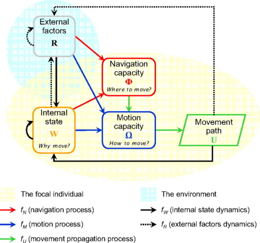
Figure 2 from Nathan et al. (2008). Conceptual diagram of questions involved in movement modeling.
- Why move? Is there a physiological or psychological state that requires moving?
- How to move? What is required? Walking, flying, or swimming?
- When (initiation and cessation) and where (direction and position) to move? What is a species ability to orient in space and time?
- What are external restrictions (resources, landscapes, predators, etc.) to movement?
- Where did the animal move? What habitats did they associate with?
- What was the probability of movement and survival?
These factors have been examined in four types of models:
- Cognitive processes
- Optimality theories
- Comparisons with random
- Biomechanical
In recent years, R packages have become a primary tool for analyzing tracking data and creating movement models. A recent paper by Joo et al. (2019) describes the many R packages available for the different stages of modeling and for a variety of biologging and tracking devices. We have listed relevant R packages under each type of movement model. For more information on other tools for data cleaning, visualization, and analyzing tracking and biologging data, see Joo et al. (2019).
What data are available?
The type of model that should be used depends upon the type of data you are working with, and the questions you have. The following types of data are often available.
- Observations of occurrence. These data are typically observations of an animal’s occurrence without being able to identify individuals across space and time. They can help us determine the distribution of a species, and the timing when a species moves through a place, but they aren’t as useful for understanding migratory connectivity of populations or individual-level drivers of movements. An example of this type of data is eBird observations of birds.
- Repeat observations of marked individuals. These data are typically point locations, repeated sampling of the same individual, and sample movements over a long time period. For example, birds that are banded on the breeding grounds and caught during migration at a banding station. Or, animals with unique markings that are recorded by different camera traps.
- Serial locations. These data are typically available more frequently than mark-recapture data and constitute time series of animal movements that give us unique insights into the lives of animals on a continuous basis. Movement tracks from electronic tags, frequent resights, and serial sets of observations of the same individual often compose this data type.
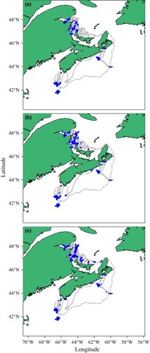
Figure 3 from Whoriskey et al. (2017). Example of path reconstruction using a Hidden Markov Model with moveHMM.
Path Reconstruction
Researchers commonly hope to create paths from discrete observations in tracking data that often come with location error or data gaps. There are several modeling methods that can be used for path reconstruction, which should be chosen based on the species, data type, and statistical assumptions.
R packages available for path reconstruction include (summarized from Joo et al. 2019):
- BayesianAnimalTracker: Bayesian Brownian bridge model
- crawl, moveHMM, kftrack, ukfsst/kfsst, argosTrack, bsam foieGras: state-space models
- ctmcmove: functional movement models
- ctmm: continuous Markov chain in gridded space
- TrackReconstruction: reconstruct tracks from magnetometer, accelerometer, depth, and speed data
Geolocator Data Processing
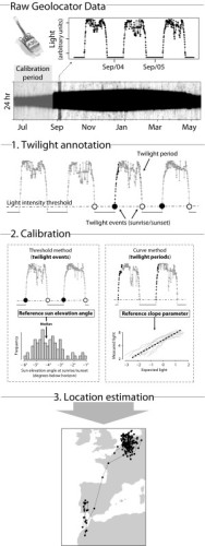
Figure 3 from Lisovski et al. (2020). Overview of analytical steps for preparing and processing data from geolocators.
Some data sources require pre-processing to get the data into a useable format for analyses. This is true especially for geolocators, which record light levels that must be converted into location estimates. A recent paper by Lisovski et al. (2020) outlines how to process and analyze geolocator data, including an online manual with example code.
Geolocator data processing can be broken down into two general methods, both of which determine location using twilight times and periods. These two methods are known as threshold and curve-fitting methods. The choice of which method is right for your project depends on many factors including the research question, the type of tag, the animal’s life history and behavior, and research constraints like time and expertise (see Lisovski et al. 2020 for a detailed discussion of methods).
Available tools for processing geolocator data include (summarized from Figure 2 in Lisovski et al. 2020):
- TAGS (online platform): threshold-based analysis, twilight annotation, extract twilight periods, calibrate data
- FLightR (R package): curve-fitting analysis, extract twilight periods, calibrate data, and refine locations
- GeoLight (R package): threshold-based analysis, twilight annotation, extract twilight periods, calibrate data, refine locations
- probGLS (R package): threshold-based analysis, refine locations
- SGAT (R package): threshold and curve-fitting analysis, calibrate data, refine locations
- TwGeos (R package): twilight annotation, extract twilight periods, calibrate data
Home Range Models
Determining an animal’s home range was one of the first questions in animal ecology and remains relevant today. In 1943, William Burt first defined the home range as, “that area traversed by the individual in its normal activities of food gathering, mating, and caring for young. Occasional sallies outside the area, perhaps exploratory in nature, should not be considered as in part of the home range.” Are there places where an animal spends more time than others? Every data set and organism is unique, thus choice of a home range model needs to be based on a comprehensive evaluation of movement and to place it in a broader context (ecology, life history, and physiology of your species). There are many types of home range analyses that can be chosen based on the questions to be addressed and the data available.
Utilization Distributions
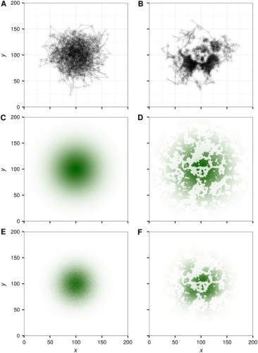
Figure 1 from Signer et al. (2017). Example of a utilization distribution created from simulated movement data using a step-selection function.
Utilization distributions are one method of estimating home ranges and can be calculated multiple ways. Utilization distributions are models that summarize space use as a continuous and probabilistic process (probability density function) whereas other home range estimation techniques (for example, Minimum Convex Polygon) may not make a distinction between places within the home range that are used more often than others by the animal. These models require the ability to appropriately define home ranges (Worton 1989).
R packages available for home range modeling include (summarized from Joo et al. 2019):
- adehabitatHR: Minimum Convex Polygon (MCP), Utilization Distribution (UD), and Kernel methods
- amt: MCP, local convex hull (LoCoh), kernel UD, and step-selection functions
- bbmm, movementAnalysis, and mkde: Brownian Bridge movement models
- ctmm: continuous time movement models (account for spatial autocorrelation and periodicity in space use). Find more information about ctmm here.
- move: dynamic Brownian Bridge movement models
- rhr: non-movement based home ranges, MCP, kernel UD, LoCoh, Brownian Bridge kernel method
- T-LoCoH: time local convex hull
Relevant MCP publications:
Using ctmm to estimate home ranges and utilization distributions for three loon species: Poessel et al. (2020)
Using adehabitatHR to estimate home ranges of common nighthawks: Ng et al. (2018)
Resource Selection Spatial Movement Models
One approach to movement modeling is to examine resource selection among individuals in a spatial array. Manly et al. (2002) introduced this concept, where resources (for example land cover categories) are analyzed according to their use by animals relative to their availability. This generally involves incorporation of GIS into models and the following components:
- Sampling at the individual or population level
- Estimating resource use or nonuse
- Quantifying resource availability
- Relating resource use to availability
R packages available for resource selection based on tracking data include (summarized from Joo et al. 2019):
- amt: resource selection functions and step-selection functions
- ctmcmove: generalized linear models
- hab (uses functions in adehabitatHS, adehabitatHR, and adehabitatLT): step-selection functions
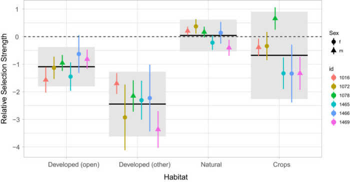
Figure 3 from Signer et al. (2018) based on Avgar et al. (2017). Example of relative selection estimates for different land cover types using a resource selection model in the package amt.
Behavioral Pattern Identification
Movement data are also useful for analyzing behavior, commonly through state space models and Hidden Markov models. These methods use data such as locations, distance, speed, and turning angles to classify behaviors. Joo et al. (2019) classifies these into three methods, summarized here: non-sequential classification or clustering, segmentation, and Hidden Markov models.
Non-sequential classification or clustering: This method classifies each fix as a type of behavior, independent of the classification of the preceding fix.
R packages available for this method include (summarized from Joo et al. 2019):
- EMbC: Expectation-maximization binary clustering
- m2b: Random forest
Segmentation methods: This method identifies changes in behavior within segments of the track.
R packages available for this method include (summarized from Joo et al. 2019):
- adehabitatLT
- bcpa: behavioral change point analysis
- marcher: mechanistic range shift analysis
- migrateR: net displacement models
- segclust2d
Hidden Markov models: This method is based on non-observed behaviors as a hidden state Markov process, which conditions the observed movement patterns.
R packages available for this method include (summarized from Joo et al. 2019):
- bsam: Bayesian sate-space model
- lsmnsd, momentuHMM, moveHMM: Hidden Markov models
-
- Figure 8 from Garriga et al. (2016). Example of behavioral pattern identification using EMbC for an Osprey migratory pathway.
-

- Figure 1 from Spitz et al. (2017). Example of behavioral pattern identification using net squared displacement (NSD) in the package migrateR.
-
- Figure 3 from Jonsen et al. (2016). Example of behavioral pattern identification for seals using Bayesian state-space models in the package bsam.
Modeling Migratory Connectivity
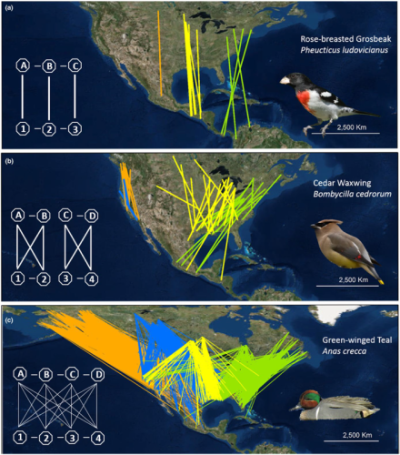
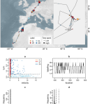
Figure 1 from Cohen et al. (2017). Three patterns of migratory connectivity shown using banding and re-encounter data for three North American species.
Though not explicitly movement modeling, analytical advances now allow researches to quantify the strength of migratory connectivity between populations. Data sources can include tracking datasets or resighting of marked individuals during different stages of the annual cycle. There are several methods available to quantify the strength of migratory connectivity:
- Mantel correlation (rM)
- Migratory Connectivity (MC): described in Cohen et al. (2017) with associated R package, MigConnectivity.
- Population spread
Relevant MCP publications:
Estimating migratory connectivity when re-encounter probabilities are heterogeneous: Cohen et al. (2014)
Quantifying the strength of migratory connectivity: Cohen et al. (2017)
Edited by Matthew Johnson (USGS Forest and Rangeland Ecosystem Science Center, matthew_johnson@usgs.gov) and Dylan Kesler (University of Missouri, keslerd@missouri.edu), 2014
Updated by Allison Huysman and Autumn-Lynn Harrison (Migratory Connectivity Project), 2020
References
- Avgar, T., Lele, S. R., Keim, J. L., and M.S. Boyce. 2017. Relative selection strength: Quantifying effect size in habitat‐and step‐selection inference. Ecology and Evolution 7: 5322–5330.
- Boulet, M. and D.R. Norris. 2006. The past and present of migratory connectivity. Ornithological Monographs 61:1-13.
- Burt, W.H. 1943. Territoriality and home range concepts as applied to mammals. Journal of Mammology 24(3): 346-352.
- Cohen, E.C., J.A. Hostetler, M.T. Hallworth, C.S. Rushing, T.S. Sillett, and P.P. Marra. 2017. Quantifying the strength of migratory connectivity. Methods in Ecology and Evolution 9: 513-524.
- Garriga J., J.R.B. Palmer, A. Oltra, and F. Bartumeus. 2016. Expectation-Maximization Binary Clustering for Behavioural Annotation. PLoS ONE 11(3): e0151984.
- Joo, R., M.E. Boone, T.A. Clay, S.C. Patrick, S. Clusella-Trullas, and M. Basille. 2019. Navigating through the R packages for movement. Journal of Animal Ecology 89:248-267.
- Jonsen, I. 2016. Joint estimation over multiple individuals improves behavioral state inference from animal movement data. Scientific Reports 6:20625.
- Lisovski, S., S. Bauer, M. Briedis, S.C. Davidson, K.L. Dhanjal-Adams, M.T. Hallworth, J. Karagicheva, C.M. Meier, B. Merkel, J. Ouwehand, L. Pedersen, E. Rakhimberdiev, A. Roberto-Charron, N.E. Seavy, M.D. Sumner, C.M. Taylor, S.J. Wotherspoon, and E.S. Bridge. 2020. Light-level geolocator analysis: A user’s guide. Journal of Animal Ecology 89:221-236.
- Manly, B.F.J., L.L. McDonald, D.L. Thomas, T.L. McDonald, and W.P. Erickson. 2002. Resource selection by animals: statistical design and analysis for field studies. Second edition. Kluwer Academic Publishers, Boston, Massachusetts, USA.
- Nathan, R., W.M. Getz, E. Revilla, M. Holyoak, R. Kadmon, D. Saltz, and P.E. Smouse. 2008. A movement ecology paradigm for unifying organismal movement research. Proceedings of the National Academy of Sciences of the United States of America 105:19052-19059.
- Ng, J. W., E. C. Knight, A. L. Scarpignato, A.-L. Harrison, E. M. Bayne, and P. P. Marra. 2018. First full annual cycle tracking of a declining aerial insectivorous bird, the common nighthawk (Chordeiles minor), identifies migration routes, nonbreeding habitat, and breeding site fidelity. Canadian Journal of Zoology 96:869–875.
- Poessel, S. A. ,B. D. Uher-Koch, J. M. Pearce, J. A. Schmutz, A.-L. Harrison, D. C. Douglas, V. R. von Biela, and T. E. Katzner. 2020. Movement and habitat use of loons for assessment of conservation buffer zones in the Arctic Coastal Plain of northern Alaska. Global Ecology and Conservation 22: e00980.
- Ramenofsky and J.C. Wingfield. 2007. Regulation of migration. Bioscience 57: 135-143.
- Signer, J., J. Fieberg, and T. Avgar. 2017. Estimating utilization distributions from fitted step-selection functions. Ecosphere 8(4):e01771.
- Signer, J., J. Fieberg, and T. Avgar. 2018. Animal movement tools (amt): R package for managing tracking data and conducting habitat selection analysis. Ecology and Evolution 9:880-890.
- Spitz, D.B, M. Hebblewhite, and T.R. Stephenson. 2017. ‘MigrateR’: extending model-driven methods for classifying and quantifying animal movement behavior. Ecography 40:788-799.
- Whoriskey, K., M. Auger-Méthé, C.M. Albertsen, F.G. Whoriskey, T.R. Binder, C.C. Krueger, and J. Mills Flemming. 2017. A hidden Markov movement model for rapidly identifying behavioral states from animal tracks. Ecology and Evolution 7:2112-2121.
- White, G.C. and Garrott, R.A. 1990. Analysis of wildlife radio-tracking data. Academic Press, San Diego, California, USA.
- Worton, B.J. 1989. Kernel methods for estimating the utilization distribution in home-range studies. Ecology 70(1): 164-168.
HOME | satellite telemetry | acoustic telemetry | geolocators | radio telemetry | motus wildlife tracking system
individual marking | molecular markers | stable isotopes | movement models | future methods